Matrices in Ruby
This semester, I have taken on a module taught using Python + numpy + various packages, which I am learning as I go. In this and later posts, I shall explore how the Python stuff can be replicated in Ruby.
I am not interested in "notebook" environments. My explorations will be
conducted in irb.
1. Matrices
Ruby has a matrix library, built-in. However, for faster performance, other libraries are available: I shall use numo-narray-alt and numo-linalg-alt. These libraries are supported by yoshoku, the developer of the Ruby machine-learning library rumale.
Once installed:
irb(main):001> require "numo/narray"
=> true
irb(main):003> Numo::NArray::VERSION
=> "0.10.0"
1.1. Creating arrays
A numo array can be created from a Ruby array:
irb(main):006> a = Numo::NArray[1,3,6,10]
=>
Numo::Int32#shape=[4]
...
irb(main):007> p a
Numo::Int32#shape=[4]
[1, 3, 6, 10]
=>
Numo::Int32#shape=[4]
[1, 3, 6, 10]
Creating a 1D and 2D array of random integers:
irb(main):020> Numo::Int32.new(4).rand(5)
=>
Numo::Int32#shape=[4]
[3, 4, 2, 4]
irb(main):021> Numo::Int32.new(2,3).rand(5)
=>
Numo::Int32#shape=[2,3]
[[2, 4, 3],
 [3, 0, 3]]
1.2. Array indexing
(output has been abbreviated)
# create sequence of 12 integers
irb(main):035> c = Numo::Int32.new(12).seq

# extract first four elements
irb(main):036> c[0...4]
[0, 1, 2, 3]
irb(main):037> c[0..3]
[0, 1, 2, 3]

# extract every other element from first four elements
irb(main):038> c[(0..3).step(2)]
[0, 2]

# extract every third element, starting from first
irb(main):039> c[(0..).step(3)]
[0, 3, 6, 9]

# extract every other element, starting from second
irb(main):040> c[(1..).step(2)]
[1, 3, 5, 7, 9, 11]

# extract elements in reverse, from index 5
irb(main):044> c[(0..5)].reverse
[5, 4, 3, 2, 1, 0]
Similarly for multi-dimensional slices:
irb(main):045> x = Numo::Int32.new(3,4).rand(12)
=>
Numo::Int32#shape=[3,4]
[[11, 0, 1, 5],
 [9, 2, 1, 7],
 [10, 10, 3, 0]]
irb(main):052> x[1...2,0...2]
=>
Numo::Int32(view)#shape=[1,2]
[[9, 2]]
1.3. Reshaping/splitting/joining arrays
Reshaping lets us convert a 1D array into a 2D one:
irb(main):057> d = c.reshape(3,4)
irb(main):058> d
Numo::Int32#shape=[3,4]
[[0, 1, 2, 3],
 [4, 5, 6, 7],
 [8, 9, 10, 11]]
For combining matrices, there is concatenate, using axis to control which
dimension the concatenation is performed along:
irb(main):095> a = Numo::Int32[[1,2], [3,4]]
irb(main):096> b = Numo::Int32[[5,6]]
irb(main):097> a
[[1, 2],
 [3, 4]]
irb(main):098> b
[[5, 6]]
irb(main):099> a.concatenate(b)
[[1, 2],
 [3, 4],
 [5, 6]]
irb(main):101> a.concatenate(b.transpose, axis:1)
[[1, 2, 5],
 [3, 4, 6]]
For dividing matrices, there is split, again using axis to determine
how the matrix is subdivided:
irb(main):075> d
[[0, 1, 2, 3],
 [4, 5, 6, 7],
 [8, 9, 10, 11]]

irb(main):103> d.split(2) # axis:0
=>
[Numo::Int32(view)#shape=[2,4]
[[0, 1, 2, 3],
 [4, 5, 6, 7]],
 Numo::Int32(view)#shape=[1,4]
[[8, 9, 10, 11]]]
irb(main):104> d.split(2, axis:1)
=>
[Numo::Int32(view)#shape=[3,2]
[[0, 1],
 [4, 5],
 [8, 9]],
 Numo::Int32(view)#shape=[3,2]
[[2, 3],
 [6, 7],
 [10, 11]]]
1.4. Scalar operations
These are applied to individual elements of the array, preserving its structure:
irb(main):105> a = Numo::Int32[10, 15, -2, 9]
irb(main):107> b = Numo::Int32.new(4).seq

irb(main):110> 2*a
[20, 30, -4, 18]
irb(main):111> a*2
[20, 30, -4, 18]
irb(main):112> b**2
[0, 1, 4, 9]
irb(main):122> a.abs
[10, 15, 2, 9]
irb(main):123> a+4
[14, 19, 2, 13]
irb(main):124> a-3
[7, 12, -5, 6]
irb(main):125> -a
[-10, -15, 2, -9]
irb(main):126> a % 2
[0, 1, 0, 1]
1.5. Operations on two matrices
irb(main):108> a+b
[10, 16, 0, 12]
irb(main):109> a-b
[10, 14, -4, 6]
irb(main):127> a.gt b
[1, 1, 0, 1]
irb(main):129> a.ge b
[1, 1, 0, 1]
irb(main):132> a.lt b
[0, 0, 1, 0]
irb(main):133> a.le b
[0, 0, 1, 0]
The comparison operations, like gt, return 1 if the corresponding elements
match the condition, else 0.
In the following, notice that * performs element-wise multiplication and
dot performs matrix multiplication:
irb(main):002> a = Numo::Int32[[2,3],[5,-8]]
irb(main):003> b = Numo::Int32[[1,-4],[8,-6]]
irb(main):004> a+b
[[3, -1],
 [13, -14]]
irb(main):005> a*b
[[2, -12],
 [40, 48]]
irb(main):006> a.dot b
[[26, -26],
 [-59, 28]]
1.6. Single matrix operations
These take a matrix and convert it to another matrix or scalar:
irb(main):117> m = Numo::Int32[[2,3],[5,-8]]
irb(main):118> m.sum
=> 2
irb(main):119> m.min
=> -8
irb(main):120> m.max
=> 5
irb(main):129> m.diagonal
[2, -8]
irb(main):130> m.trace
=> -6
and, using the numo-linalg-alt library:
irb(main):002> require "numo/linalg"
irb(main):004> Numo::Linalg.inv(m)
=>
Numo::DFloat#shape=[2,2]
[[0.258065, 0.0967742],
 [0.16129, -0.0645161]]
irb(main):005> Numo::Linalg.det(m)
=> -31.0
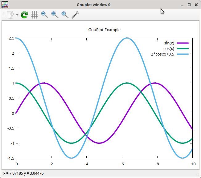
2. Graph Plotting
The final part was about plotting a graph using matplotlib, for
which Ruby is well served by the gnuplot gem:
require "gnuplot"

Gnuplot.open do |gp|
  Gnuplot::Plot.new( gp ) do |plot|

    plot.xrange "[0:10]"
    plot.title  "GnuPlot Example"

    plot.data << Gnuplot::DataSet.new( "sin(x)" ) do |ds|
      ds.with = "lines"
      ds.linewidth = 4
    end

    plot.data << Gnuplot::DataSet.new( "cos(x)" ) do |ds|
      ds.with = "lines"
      ds.linewidth = 4
    end

    plot.data << Gnuplot::DataSet.new( "2*cos(x)+0.5" ) do |ds|
      ds.with = "lines"
      ds.linewidth = 4
    end
  end
end